
Signal and systems Lab Programs
MATLAB Online Use MATLAB and Simulink through your web browserMatlab: Online Open Software Link : https://octave-online.net/#
Python: https://trinket.io/embed/python3/a5bd54189b
Python: https://colab.research.google.com/notebooks/intro.ipynb
1.Basic Operations on Matrices
Code :
clc;
close all;
clear all;
a=[1 2 -9 ; 2 -1 2; 3 -4 3];
b=[1 2 3; 4 5 6; 7 8 9];
disp('The Matrix a= ');
a
disp('The Matrix b= ');
b
c=a+b; % To find sum of a and b
disp('The Sum of a and b is ');
c
d=a-b; % To find difference of a and b
disp('The Difference of a and b is ');
d
e=a*b; % To find multiplication of a and b
disp('The Product of a and b is ');
e
Python Code for Matrices
2. Generation of Basic Continuous/Discrete Time Signals.
Code :
%Unit Impulse
clc;
clear all;
close all;
t=-10:1:10;
x=(t==0);
subplot(2,1,1);
plot(t,x,'g');
xlabel('time'); ylabel('amplitude');
title('unit impulse function'); subplot(2,1,2);
stem(t,x,'r');
xlabel('time'); ylabel('amplitude');
title('unit impulse discreat function');
%Unit step function%
clc;
clear all;
close all;
N=100;
t=1:100;
x=ones(1,N);
subplot(2,1,1);
plot(t,x,'g');
xlabel('time'); ylabel('amplitude'); title('unit step function');
subplot(2,1,2);
stem(t,x,'r');
xlabel('time'); ylabel('amplitude');
title('unit step discreat function');
%Unit Ramp signal%
clc;
clear all;
close all;
t=0:20;
x=t;
subplot(2,1,1);
plot(t,x,'g');
xlabel('time'); ylabel('amplitude'); title('unit ramp function'); subplot(2,1,2);
stem(t,x,'r');
xlabel('time'); ylabel('amplitude');
title('unit ramp discreat function');
%sinusoidal function%
clc;
clear all;
close all;
t=0:0.01:2;
x=sin(2*pi*t);
subplot(2,1,1);
plot(t,x,'g');
xlabel('time');
ylabel('amplitude');
title('sinusoidal signal');
subplot(2,1,2);
stem(t,x,'r');
xlabel('time');
ylabel('amplitude');
title('sinusoidal sequence');
%square wave%
clc;
clear all;
close all;
t=0:0.01:2;
x=square(2*pi*t);
subplot(2,1,1);
plot(t,x,'g');
xlabel('time');
ylabel('amplitude');
title('square signal');
subplot(2,1,2);
stem(t,x,'r');
xlabel('time');
ylabel('amplitude');
title('square sequence');
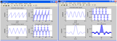
%sawtooth function%
clc;
clear all;
close all;
t=0:0.01:2;
x=sawtooth(2*pi*5*t);
subplot(2,1,1);
plot(t,x,'g');
xlabel('time');
ylabel('amplitude');
title('sawtooth signal');
subplot(2,1,2);
stem(t,x,'r');
xlabel('time');
ylabel('amplitude');
title('sawtooth sequence');
%Traingular function%
clc;
clear all;
close all; t=0:0.01:2;
x=sawtooth(2*pi*5*t,1/2);
subplot(2,1,1);
plot(t,x,'g');
xlabel('time');
ylabel('amplitude');
title('trianguler signal');
subplot(2,1,2);
stem(t,x,'r');
xlabel('time');
ylabel('amplitude');
title('trianguler sequence');
%sinc function%
clc;
clear all;
close all;
t=linspace(-5,5);
x=sinc(t);
subplot(2,1,1);
plot(t,x,'g');
xlabel('time');
ylabel('amplitude');
title('sinc signal');
subplot(2,1,2);
stem(t,x,'r');
xlabel('time');
ylabel('amplitude');
title('sinc sequence')
Python Code for Sine Wave


3. Operations on Continuous / Discrete Time Signals.
Code :
clear all;
close all;
t=0:.01:1;
% generating two input signals
x1=sin(2*pi*4*t);
x2=sin(2*pi*8*t);
subplot(2,2,1);
plot(t,x1);
xlabel('time'); ylabel('amplitude');
title('signal1:sine
wave of frequency 4Hz');
subplot(2,2,2);
plot(t,x2);
xlabel('time');
subplot(4,1,3);
ylabel('amplitude');
title('signal2:sine
wave of frequency 8Hz');
% addition of signals
y1=x1+x2;
subplot(2,2,3);
plot(t,y1);
xlabel('time'); ylabel('amplitude');
title('resultant
signal:signal1+signal2');
% multiplication of signals
y2=x1.*x2;
subplot(2,2,4);
plot(t,y2);
xlabel('time'); ylabel('amplitude');
title('resultant
signal:dot product of signal1 and signal2');
% scaling of a signal1
A=10;
y3=A*x1;
figure;
subplot(2,2,1);
plot(t,x1);
xlabel('time'); ylabel('amplitude');
title('sine wave of
frequency 4Hz')
subplot(2,2,2);
plot(t,y3);
xlabel('time'); ylabel('amplitude'); title('amplified
input signal1 ');
% folding of a signal1
l1=length(x1);
nx=0:l1-1;
subplot(2,2,3);
plot(nx,x1);
xlabel('nx'); ylabel('amplitude');
title('sine wave of
frequency 4Hz')
y4=fliplr(x1);
nf=-fliplr(nx);
subplot(2,2,4);
plot(nf,y4);
xlabel('nf'); ylabel('amplitude');
title('folded
signal');
%shifting of a signal figure;
t1=0:.01:pi;
x3=8*sin(2*pi*2*t1);
subplot(3,1,1);
plot(t1,x3); xlabel('time t1'); ylabel('amplitude');
title('sine wave of
frequency 2Hz');
subplot(3,1,2);
plot(t1+10,x3); xlabel('t1+10'); ylabel('amplitude'); title('right shifted
signal'); subplot(3,1,3);
plot(t1-10,x3);
xlabel('t1-10'); ylabel('amplitude'); title('left shifted
signal');
%operations on sequences
n1=1:1:9;
s1=[1 2 3 0 5 8 0 2 4];
figure; subplot(2,2,1);
stem(n1,s1);
xlabel('n1'); ylabel('amplitude'); title('input
sequence1');
n2=-2:1:6;
s2=[1 1 2 4 6 0 5 3 6];
subplot(2,2,2);
stem(n2,s2);
xlabel('n2'); ylabel('amplitude'); title('input
sequence2');
% addition of sequences
s3=s1+s2; subplot(2,2,3);
stem(n1,s3);
xlabel('n1'); ylabel('amplitude'); title('sum of two
sequences');
% multiplication of sequences
s4=s1.*s2;
subplot(2,2,4);
stem(n1,s4);
xlabel('n1'); ylabel('amplitude');
title('product of
two sequences');
% scaling of a sequence figure;
subplot(2,2,1);
stem(n1,s1);
xlabel('n1'); ylabel('amplitude'); title('input
sequence1');
s5=4*s1; subplot(2,2,2);
stem(n1,s5);
xlabel('n1'); ylabel('amplitude'); title('scaled
sequence1');
subplot(2,2,3);
stem(n1-2,s1);
xlabel('n1'); ylabel('amplitude');
title('left shifted
sequence1'); subplot(2,2,4); stem(n1+2,s1);
xlabel('n1'); ylabel('amplitude');
title('right shifted
sequence1');
% folding of a sequence
l2=length(s1); nx1=0:l2-1;
figure; subplot(2,1,1);
stem(nx1,s1);
xlabel('nx1'); ylabel('amplitude');
title('input
sequence1');
s6=fliplr(s1);
nf2=-fliplr(nx1); subplot(2,1,2);
stem(nf2,s6);
xlabel('nf2'); ylabel('amplitude'); title('folded
sequence1');
z1=input('enter the input sequence');
e1=sum(abs(z1).^2);
e1
% program for energy of a signal
t=0:pi:10*pi;
z2=cos(2*pi*50*t).^2;
e2=sum(abs(z2).^2);
e2
% program for power of a saequence
p1= (sum(abs(z1).^2))/length(z1);
p1
% program for power of a signal
p2=(sum(abs(z2).^2))/length(z2);
p2

Exp -4
Convolution on Continuous/Discrete Time Signals
Code
clc;
close all;
clear all;
%program for convolution of two
sequences
x=input('enter input
sequence');
h=input('enter impulse
response');
y=conv(x,h);
subplot(3,1,1); stem(x); xlabel('n');
ylabel('x(n)'); title('input signal')
subplot(3,1,2); stem(h); xlabel('n');
ylabel('h(n)'); title('impulse
response')
subplot(3,1,3); stem(y);
xlabel('n');
ylabel('y(n)'); title('linear
convolution')
disp('The resultant
signal is'); disp(y)
%program for signal convolution
t=0:0.1:10;
x1=sin(2*pi*t); h1=cos(2*pi*t);
y1=conv(x1,h1); figure; subplot(3,1,1);
plot(t,x1);
xlabel('t');
ylabel('x(t)'); title('input signal')
subplot(3,1,2);
plot(t,h1);
xlabel('t');
ylabel('h(t)'); title('impulse
response')
subplot(3,1,3); plot(y1);
xlabel('n');
ylabel('y(n)');
title('linear
convolution');

Exp-5
Even & Odd parts and Real & Imaginary parts of a Signal.
Code
clc;
close all;
clear all;
% Even and odd parts of a signal
t=0:.005:4*pi;
x=sin(t)+cos(t);
% x(t)=sint(t)+cos(t);
subplot(2,2,1)
plot(t,x)
xlabel('t');
ylabel('amplitude')
title('input signal')
y=sin(-t)+cos(-t);
%y=x(-t);
subplot(2,2,2)
plot(t,y)
xlabel('t');
ylabel('amplitude')
title('input signal with t=-t')
z=x+y;
subplot(2,2,3)
plot(t,z/2)
xlabel('t');
ylabel('amplitude');
title('even part of the signal');
%assigning a name to the plot
p=x-y;
subplot(2,2,4)
plot(t,p/2)
xlabel('t');
ylabel('amplitude');
title('odd part of the signal');
% Even and odd parts of Imaginary signals
clc;
close all;
clear all;
z=[0,2+1i*4,-3+1i*2,5-1i*1,-2-1i*4,-1i*3,0]; n=-3:3;
% plotting real and imginary parts of the sequence
figure;
subplot( 2,1,1);
stem(n,real(z));
xlabel('n');
ylabel('amplitude');
title('real part of the complex sequence');
subplot( 2,1,2);
stem(n,imag(z));
xlabel('n');
ylabel('amplitude');
title('imaginary part of the complex sequence');
zc=conj(z);
zc_folded= fliplr(zc);
zc_even=.5*(z+zc_folded);
zc_odd=.5*(z-zc_folded);
% plotting even and odd parts of the sequence
figure;
subplot( 2,2,1);
stem(n,real(zc_even));
xlabel('n');
ylabel('amplitude');
title('real part of the even sequence');
subplot( 2,2,2);
stem(n,imag(zc_even));
xlabel('n');
ylabel('amplitude');
title('imaginary part of the even sequence');
subplot( 2,2,3);
stem(n,real(zc_odd));
xlabel('n');
ylabel('amplitude');
title('real part of the odd sequence');
subplot( 2,2,4);
stem(n,imag(zc_odd));
xlabel('n');
ylabel('amplitude');
title('imaginary part of the odd sequence');

Auto Correlation and Cross Correlation on Continuous/Discrete Time Signals.
Code
clc;
close all;
clear all;
% two input sequences
x=input('enter input
sequence');
h=input('enter the
impulse suquence');
subplot(2,2,1);
stem(x); xlabel('n');
ylabel('x(n)'); title('input
sequence'); subplot(2,2,2); stem(h);
xlabel('n');
ylabel('h(n)'); title('impulse
signal');
% cross correlation between two
sequences
y=xcorr(x,h);
subplot(2,2,3); stem(y); xlabel('n');
ylabel('y(n)');
title(' Cross
Correlation between two sequences ');
fprintf('the cross correlation of above
sequences is')
disp(y)
% auto correlation of input
sequence
z=xcorr(x,x);
subplot(2,2,4); stem(z); xlabel('n');
ylabel('z(n)');
title('auto
correlation of input sequence');
fprintf('the Auto
Correlation of above sequences is')
disp(z)
% cross correlation between two
signals
% generating two input signals
t=0:0.2:10;
x1=3*exp(-2*t); h1=exp(t);
figure; subplot(2,2,1);
plot(t,x1);
xlabel('t');
ylabel('x1(t)'); title('input signal'); subplot(2,2,2);
plot(t,h1);
xlabel('t');
ylabel('h1(t)'); title('impulse
signal');
% cross correlation
subplot(2,2,3); z1=xcorr(x1,h1);
plot(z1); xlabel('t');
ylabel('z1(t)'); title('cross
correlation ');
% auto correlation
subplot(2,2,4); z2=xcorr(x1,x1);
plot(z2); xlabel('t');
ylabel('z2(t)'); title('auto
correlation ');
Output:
enter input sequence[1 2 5 7]
Enter the
impulse suquence[2 6 0 5 3]
The cross correlation of above sequences is 3.0000 11.0000 25.0000 52.0000 49.0000 34.0000 52.0000 14.0000 0.0000
The Auto Correlation of above sequences is 7.0000 19.0000 47.0000 79.0000 47.0000 19.0000 7.0000

Exp-7
Verification of Linearity and Time Invariance Properties of a Given System.
Code
% Linearity%
% conv((a1*x1(n)+a2*x2(n)),h(n))=LHS
% (a1*conv(x1(n),h(n)))+(a2*conv(x2(n),h(n)))=RHS
clc;
clear all;
close all;
% entering two input sequences and impulse sequence
x1 = input (' type the samples of x1 ');
x2 = input (' type the samples of x2 ');
if(length(x1)~=length(x2))
disp('error: Lengths of x1 and x2 are different');
return;
end
h = input (' type the samples of h ');
% length of output sequence
N = length(x1) + length(h) -1;
disp('length of the output signal will be ');
disp(N);
% entering scaling factors
a1 = input (' The scale factor a1 is ');
a2 = input (' The scale factor a2 is ');
LHS = conv(a1 * x1 + a2 * x2,h);% LHS= conv((a1*x1(n)+a2*x2(n)),h(n))
RHS = (a1 * conv(x1,h)) + (a2 * conv(x2,h)); % RHS= a1*conv(x1(n),h(n))+a2*conv(x2(n),h(n))
disp ('Input signal x1 is ');
disp(x1);
disp ('Input signal x2 is ');
disp(x2);
disp ('Output Sequence LHS is ');
disp(LHS);
disp ('Output Sequence RHS is ');
disp(RHS);
if ( LHS == RHS )
disp(' LHS = RHS. Hence the LTI system is LINEAR ')
end
% time invariant property
% time invariant property
%TIME INVARIANT SYSTEM
% y(n-k)= T[x(n-k)]
% LOGIC
% y=conv(x,h)
% xd=x(n-d)
% RHS= conv(xd,h)
% LHS= y(n-d);
% LHS==RHS TIME INVARIANT
clc;
clear all;
close all;
x = input( ' Type the samples of signal x(n): ' );
h = input( ' Type the samples of signal h(n): ' );
d = input( ' Enter Positive Delay: ' );
y = conv(x,h); % Original response
xd = [zeros(1,d), x]; % Shifted to right by d units
RHS = conv(xd,h) % RHS T[x(n-k)]=conv(xd,h)
LHS = [zeros(1,d), y] % LHS delay the output sequence by k samples
nxd = 0:length(xd)-1;
nyd = 0:length(RHS)-1;
nyp = 0:length(LHS)-1;
subplot(2,1,1);
stem(nyd,RHS);
grid;
xlabel( ' Time Index n ' );
ylabel( ' y(n) ' );
title( ' RHS y(n,k)= T[x(n-k)] ' );
subplot(2,1,2);
stem(nyp,LHS);
grid;
xlabel( ' Time Index n ' );
ylabel( ' y(n-k) ' );
title( ' Output Signal LHS y(n-k) ' );
if (LHS==RHS)
disp('the sytem is time invariant')
end
clc;
clear all;
close all;
% entering two input sequences
x = input( ' Type the
samples of signal x(n) ' );
h = input( ' Type the
samples of signal h(n) ' );
% original response
y = conv(x,h);
disp( ' Enter a
POSITIVE number for delay ' );
d = input( ' Desired
delay of the signal is ' );
% delayed input
xd = [zeros(1,d), x];
nxd = 0 : length(xd)-1;
%delayed output
yd = conv(xd,h);
nyd = 0:length(yd)-1;
disp(' Original
Input Signal x(n) is '); disp(x);
disp(' Delayed
Input Signal xd(n) is '); disp(xd);
disp(' Original
Output Signal y(n) is '); disp(y);
disp(' Delayed
Output Signal yd(n) is '); disp(yd);
xp = [x , zeros(1,d)];
subplot(2,1,1);
stem(nxd,xp); grid;
xlabel( ' Time Index n
'
); ylabel( ' x(n) ' );
title( ' Original
Input Signal x(n) ' ); subplot(2,1,2);
stem(nxd,xd); grid;
xlabel( ' Time Index n
'
); ylabel( ' xd(n) ' );
title( ' Delayed
Input Signal xd(n) ' );
yp = [y zeros(1,d)];
figure; subplot(2,1,1);
stem(nyd,yp); grid;
xlabel( ' Time Index n
'
); ylabel( ' y(n) ' );
title( ' Original
Output Signal y(n) ' ); subplot(2,1,2);
stem(nyd,yd); grid;
xlabel( ' Time Index n
'
); ylabel( ' yd(n) ' );
title( ' Delayed
Output Signal yd(n) ' );


Exp-8
Computation of Unit Sample, Unit Step and Sinusoidal Responses of the Given LTI System.
Code
%given difference equation
y(n)-y(n-1)+.9*y(n-2)=x(n);
b=[1];
a=[1,-1,.9];
n =0:3:100;
%generating impulse signal
x1=(n==0);
%impulse response
h1=filter(b,a,x1);
subplot(3,1,1);
stem(n,h1);
xlabel('n');
ylabel('h(n)');
title('impulse
response');
%generating step signal
x2=(n>0);
% step response
s=filter(b,a,x2);
subplot(3,1,2);
stem(n,s);
xlabel('n');
ylabel('s(n)')
title('step
response');
%generating sinusoidal
signal
t=0:0.1:2*pi;
x3=sin(t);
% sinusoidal response
h2=filter(b,a,x3);
subplot(3,1,3);
stem(h2);
xlabel('n');
ylabel('h(n)');
title('sin response');
% verifing stability
figure;
zplane(b,a);


Exp-9
Synthesis of Signals Using Fourier series.
Code
% synthesis of signal using fourier series
Complete Program with function calling
clc;
clear all;
close all;
fs=100;
T=2;
w0=(2*pi)/T;
k=0:1/fs:10-1/fs;
y=square(w0*k,50);
subplot(2,2,1);
plot(k,y);
xlabel('n');
ylabel('Amplitude');
title('Input signal -Square wave to be approximated');
F=fourierseries(w0,T,fs);
subplot(2,2,2);
plot(k,F);
grid on;
hold on
plot(k,y);
xlabel('n');
ylabel('Amplitude');
title ('square wave along with approximated fourier series waveform');
legend('Fourier Approximation','Actual Function');
%New File
function F = fourierseries(w0,T,fs)
syms t
k=0:1/fs:10-1/fs;
N=10;
n=1:N;
a0=(2/T)*(int(1,t,0,1)+int(-1,t,1,2));
an=(2/T)*(int(1*cos(n*w0*t),t,0,1)+int(-1*cos(n*w0*t),t,1,2));
bn=(2/T)*(int(1*sin(n*w0*t),t,0,1)+int(-1*sin(n*w0*t),t,1,2));
F=a0/2;
for i =1:N
F=F+an(i)*cos(i*w0*k)+bn(i)*sin(i*w0*k);
end
end
Complete Program without function calling
clc;
clear all;
close all;
fs=100;
T=2;
w0=(2*pi)/T;
k=0:1/fs:10-1/fs;
y=square(w0*k,50);
figure;
plot(k,y);
xlabel('n');
ylabel('Amplitude');
title('Input signal -Square wave
to be approximated');
syms t
N=10;
n=1:N;
a0=(2/T)*(int(1,t,0,1)+int(-1,t,1,2));
an=(2/T)*(int(1*cos(n*w0*t),t,0,1)+int(-1*cos(n*w0*t),t,1,2));
bn=(2/T)*(int(1*sin(n*w0*t),t,0,1)+int(-1*sin(n*w0*t),t,1,2));
F=a0/2;
for i =1:N
F=F+an(i)*cos(i*w0*k)+bn(i)*sin(i*w0*k);
end
figure;
plot(k,F);
grid on;
hold on
plot(k,y);
xlabel('n');
ylabel('Amplitude');
title ('square wave along with
approximated fourier series waveform');
legend('Fourier
Approximation','Actual Function');


Problem
2:
fs=100;
T=2;
w0=(2*pi)/T;
k=0:1/fs:10-1/fs;
y=1+square(w0*k,50);
figure;
plot(k,y);
xlabel('n');
ylabel('Amplitude');
title('Input signal -Square wave
to be approximated');
syms t
N=10;
n=1:N;
a0=(2/T)*(int(2,t,0,1)+int(0,t,1,2));
an=(2/T)*(int(2*cos(n*w0*t),t,0,1)+int(0*cos(n*w0*t),t,1,2));
bn=(2/T)*(int(2*sin(n*w0*t),t,0,1)+int(0*sin(n*w0*t),t,1,2));
F=a0/2;
for i =1:N
F=F+an(i)*cos(i*w0*k)+bn(i)*sin(i*w0*k);
end
figure;
plot(k,F);
grid on;
hold on
plot(k,y);
xlabel('n');
ylabel('Amplitude');
title ('square wave along with
approximated fourier series waveform');
legend('Fourier
Approximation','Actual Function');
output
waveform:


Exp-10
Fourier series of a Given Signal and Plotting Its Magnitude and Phase Spectrum.
Code
syms t;
choice=input('enter your
choice(1/2/3):');
if choice==1
ft=input('enter any
function of t(one piece)')
ft=str2sym(ft);
N=input('Enter no.of
harmonics to be calculated');
t1=input('Enter first
limit');
t2=input('enter second
limit');
T=t2-t1; % time period
w0=(2*pi)/T; %Frequency
n=-N:1:N-1;% no.of
harmonics both sides
Fn=(1/T)*int((ft*exp(-1j*n*w0*t)),t1,t2);
expar=exp(1j*w0*n*t);
t=t1:0.001:t2;
t=t(:,1:end-1);
nop=length(t);
ft0=eval(ft);% actual
function of t
elseif choice==2
ft1=input('Enter any
function of t(First part)');
ft2=input('Enter any
function of t(second part)');
ft1=str2sym(ft1);
ft2=str2sym(ft2);
N=input('Enter no.of
harmoncis to be calculated');
t1=input('Enter first
limit');
t2=input('Enter seond
limit');
t3=input('Enter third
limit');
T=t3-t1;
w0=(2*pi)/T;
n=-N:1:N;
Fn=(1/T)*(int((ft1*exp(-1j*n*w0*t)),t1,t2)+int((ft2*exp(-1j*n*w0*t)),t2,t3));
expar=exp(1j*w0*n*t);
tx=t1:0.001:t3;
t=tx(:,1:end-1);
nop=length(t);
%plotting input function
nop1=find(tx==t2)-find(tx==t1);
nop2=find(tx==t3)-find(tx==t2);
t=tx(1:nop1);
ftt1=eval(ft1).*ones(1,nop1);
t=tx(nop2+1:nop);
ftt2=eval(ft2).*ones(1,nop2);
ft0=[ftt1 ftt2];
t=tx(:,1:end-1);
elseif choice==3
ft1=input('enter any
function of t(First part)');
ft2=input('Enter any
function of t(Second part)');
ft3=input('enter any
function of t(third part)');
ft1=str2sym(ft1);
ft2=str2sym(ft2);
ft3=str2sym(ft3);
N=input('enter no.of
harmonics to be calculated');
t1= input('enter first
limit');
t2=input('Enter second
limit');
t3=input('Enter third
limit');
t4=input('Enter fourth
limit');
T=t4-t1;
w0=(2*pi)/T;
n=-N:1:N;
Fn=(1/T)*(int((ft1*exp(-1j*n*w0*t)),t1,t2)+int((ft2*exp(-1j*n*w0*t)),t2,t3)+int((ft3*exp(-1j*n*w0*t)),t3,t4));
expar=exp(1j*w0*n*t);
% plotting actual function
tx=t1:0.001:t4;
t=tx(:,1:end-1);
nop=length(t);
nop1=find(tx==t2)-find(tx==t1);
nop2=find(tx==t3)-find(tx==t2);
nop3=find(tx==t4)-find(tx==t3);
t=tx(1:nop1);ftt1=eval(ft1).*ones(1,nop1);
t=tx(1:nop2+1);ftt2=eval(ft2).*ones(1,nop2);
t=tx(1:nop3+1);ftt3=eval(ft3).*ones(1,nop3);
ft0=[ftt1 ftt2 ftt3];
t=tx(:,1:end-1);
end
n0=round(length(Fn)/2);
avg=double(Fn(n0));
ftapprox=sum(expar.*Fn);
ftapprox=eval(ftapprox);
plot(t,ftapprox,t,ft0,'r','LineWidth',1);
grid on;
xlabel('Time');
ylabel('Amplitude');
title('Fourier
Approximation Plot for N harmonics')
legend('Fourier
Approximation','Actual Function');
% plotting magnitude and phase spectrum
if isreal(Fn)
mag=Fn;
thetadeg=zeros(length(Fn));
else
mag=abs(Fn);% finding
magnitude
theta=angle(Fn); %Finding pahse
thetadeg=convert2deg(eval(theta));% phase in
degrees
end
figure;
subplot(1,2,1)
stem(n,mag,'LineWidth',2);
grid on;
title('magnitude
Spectrum');
xlabel('n');
ylabel('magnitude');
subplot(1,2,2)
stem(n,thetadeg,'LineWidth',2); grid on; title('phase
Spectrum');
xlabel('n'); ylabel('Phase(Deg.)');
Command window:
enter your choice(1/2/3):1
enter any function of t(one piece)
'exp(-t)'
ft =
'exp(-t)'
Enter no.of harmonics to be
calculated 5
Enter first limit 0
enter second limit 1


Command window
enter your choice(1/2/3):2
Enter any function of t(First
part) '1'
Enter any function of t(second
part) '0'
Enter no.of harmoncis to be
calculated 5
Enter first limit 0
Enter seond limit 0.5
Enter third limit 1
Output waveform:


Command window:
enter your choice(1/2/3):3
enter any function of t(First
part) '0'
Enter any function of t(Second
part) '1'
enter any function of t(third
part) '0'
enter no.of harmonics to be
calculated 10
enter first limit -1
Enter second limit -0.5
Enter third limit 0.5
Enter fourth limit 1
Output waveform:


Exp-11
Fourier Transform of a Given Signal and Plotting Its Magnitude and Phase Spectrum.
Code
%Fourier &
Inverse Fourier Transform of Exponential Signal%
clc;
clear all;
close all;
fs=1000;
N=1024; %
length of fft sequence
t=[0:N-1]*(1/fs);
% input signal
x=0.8*cos(2*pi*100*t);
subplot(3,1,1);
plot(t,x);
axis([0 0.05 -1
1]);
grid; xlabel('t');
ylabel('amplitude');
title('input signal');
% magnitude
spectrum
x1=fft(x);
k=0:N-1;
Xmag=abs(x1);
subplot(3,1,2);
plot(k,Xmag);
grid;
xlabel('t');
ylabel('amplitude'); title('magnitude of
fft signal')
%phase
spectrum
Xphase=angle(x1)*(180/pi);
subplot(3,1,3); plot(k,Xphase);
grid; xlabel('t');
ylabel('angle
in degrees'); title('phase of fft signal');
output wave
forms:

Exp-12
Laplace Transform & Inverse Laplace Transform of Some Signals.
Code
%laplace
transform of all signals
syms impsteprmpparbxytex
imp=dirac(t);
stp=heaviside(t);
rmp=t;
parb=t^2;
x=sin(2*t);
y=cos(2*t);
ex=exp(-3*t);
fprintf('the
laplace transfrom of impulse signal is \n')
laplace(imp)
fprintf('the
laplace transfrom of step signal is \n')
laplace(stp)
fprintf('the
laplace transfrom of ramp signal is \n')
laplace(rmp)
fprintf('the
laplace transfrom of parabolic signal is \n')
laplace(parb)
fprintf('the
laplace transfrom of sine signal is \n')
laplace(x)
fprintf('the
laplace transfrom of cosine signal is \n')
laplace(y)
fprintf('the
laplace transfrom of exponential signal is \n')
laplace(ex)
output:
the laplace
transfrom of impulse signal is
ans =
1
the laplace
transfrom of step signal is
ans =
1/s
the laplace
transfrom of ramp signal is
ans =
1/s^2
the laplace
transfrom of parabolic signal is
ans =
2/s^3
the laplace
transfrom of sine signal is
ans =
2/(s^2 + 4)
the laplace
transfrom of cosine signal is
ans =
s/(s^2 + 4)
the laplace
transfrom of exponential signal is
ans =
1/(s + 3)
% to find inverse
laplace transform
syms sta
f(s)=1/(s-a);
I1=ilaplace(f(s))
disp('inverse
laplace transform is')
disp(I)
f(s)=1/s^2;
I2=ilaplace(f(s))
disp('inverse
laplace transform is')
disp(I)
output:
inverse laplace
transform is
exp(a*t)
inverse laplace
transform is
t
Exp-13
Z - Transform & Inverse Z Transform of Some Signals.
Code
% finding z- transform and inverse z-
transform
syms n
f= sin(n);
z= ztrans(f);
disp('Ztransform
of sin(n)is');
disp(z);
zz=iztrans(z);
disp('displaying
inverse z transform')
disp(zz);
f2= cos(n);
z1= ztrans(f2);
disp('Ztransform
of cos(n)is');
disp(z1);
zz1=iztrans(z1);
disp('displaying
inverse z transform')
disp(zz1);
output:
Ztransform of
sin(n)is
(z*sin(1))/(z^2 -
2*cos(1)*z + 1)
displaying inverse z
transform
sin(n)
Ztransform of
cos(n)is
(z*(z -
cos(1)))/(z^2 - 2*cos(1)*z + 1)
displaying inverse z
transform
cos(n)
Exp-14
Verification of Sampling Theorem.
Code
%SAMPLING THEOREM%
clc;
clear all;
close all;
t=-10:.01:10;
T=4;
fm=1/T;
x=cos(2*pi*fm*t);
subplot(2,2,1);
plot(t,x);
xlabel('time');
ylabel('x(t)');
title('continous
time signal');
grid;
n1=-4:1:4;
fs1=1.6*fm;
fs2=2*fm;
fs3=8*fm;
x1=cos(2*pi*fm/fs1*n1);
subplot(2,2,2);
stem(n1,x1);
xlabel('time');
ylabel('x(n)');
title('discrete
time signal with fs<2fm');
hold on;
subplot(2,2,2);
plot(n1,x1);
grid;
n2=-5:1:5;
x2=cos(2*pi*fm/fs2*n2);
subplot(2,2,3);
stem(n2,x2);
xlabel('time');
ylabel('x(n)');
title('discrete
time signal with fs=2fm');
hold on;
subplot(2,2,3);
plot(n2,x2)
grid;
n3=-20:1:20;
x3=cos(2*pi*fm/fs3*n3);
subplot(2,2,4);
stem(n3,x3);
xlabel('time');
ylabel('x(n)');
title('discrete
time signal with fs>2fm')
hold on;
subplot(2,2,4);
plot(n3,x3)
grid;
Exp-15
Finding and Plotting the Poles and Zeros in S-Plane and the Corresponding Magnitude and Phase responses for the Given Transfer Function.
Code
clc;
clear all;
close all;
%enter the
numerator and denominatorcoefficients in square brackets
num=input('enter
the numerator coefficients');
den=input('enter
the denominatorcoefficients');
% ploe-zero
plot in s-plane
H1=tf(num,den) %
find transfer function H(s)
[p1,z1]=pzmap(H1);
% find the locations of poles and zeros
disp('poles
ar at ');disp(p1);
disp('zeros
ar at ');disp(z1);
figure;
%plot the
pole-zero map in s-plane
pzmap(H1);
title('pole-zero
map of LTI system in s-plane');
h2 =
freqs(den,num);
mag2= abs(h2);
figure;
plot(mag2);
title('Magnitude Response');grid on
phase2
=angle(h2);
figure;
plot(phase2);title('Phase
Response');grid on
OUTPUT:
enter the numerator
coefficients [1 -1 4 3.5]
enter the
denominatorcoefficients [2 3 -2.5 6]


Exp-16
Finding and Plotting the Poles and Zeros in Z-Plane and the Corresponding Magnitude and Phase responses for the Given Transfer Function.
Code
clc;
clear all;
close all;
%enter the
numerator and denominatorcoefficients in square brackets
num=input('enter
the numerator coefficients');
den=input('enter
the denominatorcoefficients');
%find the
transfer function using built-in function 'filt'
H=filt(num,den);
%find
locations of zeros
z=zero(H);
disp('zeros
are at '); disp(z);
%find
residues,pole locations and gain constant of H(z)
[r p
k]=residuez(num,den);
disp('poles
are at ');
disp(p);
%plot the pole
zero map in z-plane
zplane(num,den);
title('pole-zero
map of LTI system in z-plane');
h1 =
freqz(den,num);
mag= abs(h1);
figure;
plot(mag);title('Magnitude
Response'); grid on
phase
=angle(h1);
figure;
plot(phase);title('Phase
Response'); grid on
Output:
enter the
numerator coefficients[1 -1 4 3.5]
enter the
denominatorcoefficients[2 3 -2.5 6]
zeros are at
0.8402 + 2.1065i
0.8402 - 2.1065i
-0.6805 + 0.0000i
poles are at
-2.4874 + 0.0000i
0.4937 + 0.9810i
0.4937 - 0.9810i
Graphs


c